
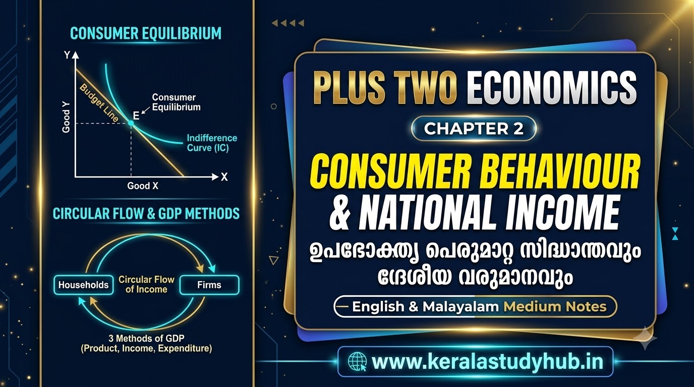
Kerala Plus Two Economics Chapter 2 Notes: Theory of Consumer Behaviour & National Income Accounting (ഉപഭോക്തൃ പെരുമാറ്റ സിദ്ധാന്തവും ദേശീയ വരുമാനവും) — DHSE Solutions & Exam Q&A PDF
- Kerala Plus Two Economics Chapter 2 Notes: Theory of Consumer Behaviour & National Income Accounting (ഉപഭോക്തൃ പെരുമാറ്റ സിദ്ധാന്തവും ദേശീയ വരുമാനവും) — DHSE Solutions & Exam Q&A PDF
- 1. Chapter Weightage & Exam Blueprint (DHSE Plus Two Economics)
- 2. PART A: Theory of Consumer Behaviour (ഉപഭോക്തൃ പെരുമാറ്റ സിദ്ധാന്തം — Microeconomics Ch 2)
- 2.1 Concept of Utility: Cardinal vs Ordinal Utility, TU vs MU & Law of DMU (Sure 4 or 5 Marks)
- 2.2 The Consumer’s Budget: Budget Set, Budget Line & Slope (ബജറ്റ് സെറ്റും ബജറ്റ് രേഖയും — Sure 3 or 4 Marks)
- 2.3 Indifference Curve (IC), Indifference Map & Consumer’s Equilibrium (നിസ്സംഗതാ വക്രവും ഉപഭോക്താവിന്റെ സന്തുലിതാവസ്ഥയും — Guaranteed 5 or 8 Marks!)
- 2.4 Demand, Law of Demand, Types of Goods & Price Elasticity of Demand (ചോദനവും ചോദനത്തിന്റെ വില ഇലാസ്തികതയും)
- 3. PART B: National Income Accounting (ദേശീയ വരുമാന അക്കൗണ്ടിംഗ് — Macroeconomics Ch 2)
- 3.1 Basic Macroeconomic Concepts: Final vs Intermediate Goods, Stocks vs Flows & Depreciation
- 3.2 Circular Flow of Income in a Two-Sector Economy (ദ്വിമേഖലാ സമ്പദ്വ്യവസ്ഥയിലെ വരുമാനത്തിന്റെ ചാക്രിക പ്രവാഹം — Sure 4 or 5 Marks)
- 3.3 Three Methods of Calculating National Income (ദേശീയ വരുമാനം കണക്കാക്കുന്ന 3 രീതികൾ — Guaranteed 8-Mark Essay!)
- 3.4 Macroeconomic Identities Conversion Rules & GDP and Welfare
- 4. 30 Solved DHSE Kerala Board Exam Questions & Answers (1, 2, 3, 4, 5 & 8 Marks)
- Part 1: 1-Mark Objective Questions (Q1 to Q10)
- Part 2: 2-Mark & 3-Mark Questions (Q11 to Q22)
- Part 3: 4-Mark, 5-Mark & 8-Mark Long Essay Questions (Q23 to Q30)
- 5. D+ (Just Pass / 30% Minimum Rule) Capsule & Sure A+ Revision Box
- 6. Teacher’s Corner: SCERT Scheme of Work, Learning Outcomes & Classroom Activities (അധ്യാപകർക്കായി)
- 7. Popular Search Queries by Kerala Students & Teachers
Welcome to Kerala Study Hub (keralastudyhub.in), your complete online learning platform for SCERT Kerala and DHSE Higher Secondary examinations. If you are a Class 12 (Plus Two) Commerce or Humanities student or teacher searching for Kerala Plus Two Economics Chapter 2 Notes: Theory of Consumer Behaviour (Part A: Microeconomics) and National Income Accounting (Part B: Macroeconomics) (ഉപഭോക്തൃ പെരുമാറ്റ സിദ്ധാന്തവും ദേശീയ വരുമാന അക്കൗണ്ടിംഗും), this master study guide is the most important resource for your board exam preparation.
Why is Chapter 2 of Microeconomics and Macroeconomics the most important milestone in Plus Two Economics? Because together, Microeconomics Chapter 2 (14 Marks) and Macroeconomics Chapter 2 (12 Marks) carry a massive 26 Marks out of 80 in the Final March DHSE Board Exam—including TWO guaranteed 8-Mark Long Essay Questions (one on Consumer Equilibrium / Indifference Curve / Law of Demand and another on the Three Methods of Calculating National Income)! In this comprehensive bilingual guide, we explain every theory, formula, schedule, and numerical problem in Simple English + Malayalam Medium (മലയാളം മീഡിയം) along with solved NCERT textbook exercises, a Teacher’s Scheme of Work Corner, and 30 solved DHSE board exam questions.
1. Chapter Weightage & Exam Blueprint (DHSE Plus Two Economics)
Look at the massive weightage of Chapter 2 in both Microeconomics and Macroeconomics in the DHSE Kerala question paper:
| Feature / Exam Parameter | Part A (Micro Ch 2): Theory of Consumer Behaviour | Part B (Macro Ch 2): National Income Accounting |
|---|---|---|
| Malayalam Title (മലയാളം) | ഉപഭോക്തൃ പെരുമാറ്റ സിദ്ധാന്തം | ദേശീയ വരുമാന അക്കൗണ്ടിംഗ് |
| Final Board Exam Weightage | 14 Marks (Highest in Microeconomics!) | 12 Marks (Highest in Macroeconomics!) |
| Total Combined Weightage | 26 Marks out of 80 (nearly 33% of the entire Economics Board Exam Paper!) | |
| Guaranteed Exam Questions | 1. Total Utility (TU) vs Marginal Utility (MU) & Law of DMU (4/5 Marks) 2. Budget Line, Budget Set & Shifts/Rotations (3/4 Marks) 3. Indifference Curve (IC) Properties & Consumer Equilibrium (5/8 Marks Essay!) 4. Law of Demand, Normal vs Inferior Goods, Substitutes vs Complements (3/4 Marks) 5. Price Elasticity of Demand Numerical Problem (3/4 Marks) |
1. Stocks vs Flows, Final vs Intermediate Goods & Depreciation (2/3 Marks) 2. Circular Flow of Income in a 2-Sector Economy (4/5 Marks) 3. Three Methods of Measuring National Income — Product, Expenditure & Income Method (Guaranteed 8-Mark Essay!) 4. GDP to NNP_FC Conversions & GDP and Welfare Limitations (4/5 Marks) |
Explore Related Plus Two & Plus One Guides on Kerala Study Hub:
- Kerala Plus Two Economics Chapter 1 Notes: Introduction to Microeconomics & Macroeconomics
- Kerala Plus One Economics Chapter 2 Notes: Indian Economy 1950–1990 & Collection of Data
- Kerala Plus Two Business Studies Chapter 2 Notes: Principles of Management
- Kerala Plus Two Accountancy Chapter 2 Notes: Admission of a Partner
- Kerala Plus Two Computer Application Chapter 1 & 2 Notes: Review of C++ & Arrays
2. PART A: Theory of Consumer Behaviour (ഉപഭോക്തൃ പെരുമാറ്റ സിദ്ധാന്തം — Microeconomics Ch 2)
2.1 Concept of Utility: Cardinal vs Ordinal Utility, TU vs MU & Law of DMU (Sure 4 or 5 Marks)
What is Utility (ഉപയുക്തത)?
Utility is the want-satisfying power of a commodity (ഒരു വസ്തുവിന് മനുഷ്യന്റെ ആവശ്യങ്ങളെ തൃപ്തിപ്പെടുത്താനുള്ള കഴിവ്). There are two approaches to studying utility:
- Cardinal Utility Analysis (കാർഡിനൽ യൂട്ടിലിറ്റി വിശകലനം — Propounded by Alfred Marshall): Assumes that utility can be measured quantitatively in exact cardinal numbers (1, 2, 3…) using an imaginary unit called ‘Utils’.
- Ordinal Utility Analysis / Indifference Curve Analysis (ഓർഡിനൽ യൂട്ടിലിറ്റി വിശകലനം — Propounded by J.R. Hicks & R.G.D. Allen): Assumes that utility is a psychological feeling that cannot be measured in exact numbers, but the consumer can rank (order) different bundles of goods according to preference (1st, 2nd, 3rd).
Total Utility (TU) vs Marginal Utility (MU):
- Total Utility (TU — മൊത്തം ഉപയുക്തത): The aggregate utility derived by a consumer from consuming a given number of units of a commodity (
TUₙ = MU₁ + MU₂ + ... + MUₙ). - Marginal Utility (MU — സീമാന്ത ഉപയുക്തത): The additional utility derived from consuming one more unit of a commodity.
Formula:MUₙ = TUₙ − TUₙ₋₁(orMU = ΔTU ÷ ΔQ).
Law of Diminishing Marginal Utility — Law of DMU (അപചയ സീമാന്ത ഉപയുക്തതാ നിയമം):
Statement: As a consumer consumes more and more units of a specific commodity continuously (keeping consumption of other goods constant), the Marginal Utility (MU) derived from each successive unit goes on diminishing (കുറഞ്ഞുവരുന്നു).
Schedule & Relationship Between Total Utility (TU) and Marginal Utility (MU) (Sure 4 Marks!):
| Units of Commodity (Q) | Total Utility (TU) | Marginal Utility (MU = TUₙ − TUₙ₋₁) | Phase / Relationship Between TU and MU |
|---|---|---|---|
| 1 | 12 | 12 | 1. As long as MU is Positive (MU > 0): TU increases at a diminishing rate. |
| 2 | 20 | 20 − 12 = 8 | |
| 3 | 25 | 25 − 20 = 5 | |
| 4 | 28 | 28 − 25 = 3 | |
| 5 (Point of Satiety) | 28 (Maximum) | 28 − 28 = 0 (Zero) | 2. When MU becomes Zero (MU = 0): TU reaches its MAXIMUM (Point of Satiety / പൂർണ്ണ സംതൃപ്തി). |
| 6 | 25 | 25 − 28 = −3 (Negative) | 3. When MU becomes Negative (MU < 0): TU starts falling (declining). |
2.2 The Consumer’s Budget: Budget Set, Budget Line & Slope (ബജറ്റ് സെറ്റും ബജറ്റ് രേഖയും — Sure 3 or 4 Marks)
Suppose a consumer has a fixed money income M which he spends on two goods—Good 1 (quantity x₁ at price P₁) and Good 2 (quantity x₂ at price P₂):
- Budget Constraint (ബജറ്റ് പരിമിതി):
P₁x₁ + P₂x₂ ≤ M(Total expenditure on the two goods cannot exceed money incomeM). - Budget Set (ബജറ്റ് സെറ്റ് / ബജറ്റ് ഗണം): The collection of all bundles of Good 1 and Good 2 that the consumer can buy with his given income
Mat prevailing market pricesP₁andP₂(i.e., all bundles satisfyingP₁x₁ + P₂x₂ ≤ M). - Budget Line / Price Line (ബജറ്റ് രേഖ): The locus of all bundles of two goods whose cost is exactly equal to the consumer’s money income.
Equation of Budget Line:P₁x₁ + P₂x₂ = M - Key Formulas on Budget Line (Frequently Asked in 1, 2 & 3 Mark Numerical Questions!):
- Horizontal Intercept (Maximum units of Good 1 when x₂ = 0):
M ÷ P₁ - Vertical Intercept (Maximum units of Good 2 when x₁ = 0):
M ÷ P₂ - Slope of the Budget Line (Price Ratio):
−P₁ ÷ P₂(Measures how many units of Good 2 must be given up in the market to buy 1 extra unit of Good 1).
- Horizontal Intercept (Maximum units of Good 1 when x₂ = 0):
- Changes in the Budget Line:
- Change in Income (M) keeping Prices constant ⇒ Parallel Shift of Budget Line: If Income
Mincreases, the Budget Line shifts parallelly to the Right (Outward); if IncomeMdecreases, it shifts parallelly to the Left (Inward). - Change in Price of one Good (P₁ or P₂) keeping Income constant ⇒ Rotation (Pivot) of Budget Line: If
P₁falls, the consumer can buy more of Good 1, so the horizontal intercept (M ÷ P₁) moves outward to the right while the vertical intercept remains fixed.
- Change in Income (M) keeping Prices constant ⇒ Parallel Shift of Budget Line: If Income
2.3 Indifference Curve (IC), Indifference Map & Consumer’s Equilibrium (നിസ്സംഗതാ വക്രവും ഉപഭോക്താവിന്റെ സന്തുലിതാവസ്ഥയും — Guaranteed 5 or 8 Marks!)
- Monotonic Preferences (മോണോടോണിക് മുൻഗണന): A consumer’s preferences are said to be monotonic if, between any two bundles, the consumer always prefers the bundle which has more of at least one of the goods and no less of the other good (e.g., preferring bundle
(4, 5)over(4, 3)). - Indifference Curve — IC (നിസ്സംഗതാ വക്രം): A curve joining all combinations (bundles) of two goods that give the consumer the exact same level of satisfaction (utility), so that the consumer is indifferent among them.
- Indifference Map (നിസ്സംഗതാ ഭൂപടം): A family or group of two or more Indifference Curves in a single graph representing different levels of satisfaction. A higher Indifference Curve always represents a higher level of satisfaction!
- Marginal Rate of Substitution — MRS (സീമാന്ത പ്രതിസ്ഥാപന നിരക്ക്): The rate at which a consumer is willing to substitute (sacrifice) Good 2 for getting one additional unit of Good 1 while keeping total satisfaction constant. It is the Slope of the Indifference Curve:
MRS = ΔY ÷ ΔX = Δx₂ ÷ Δx₁
Three Important Properties / Features of Indifference Curve (നിസ്സംഗതാ വക്രത്തിന്റെ 3 സവിശേഷതകൾ — Sure 3 or 4 Marks):
- Indifference Curve Slopes Downwards from Left to Right (ഇടത്തുനിന്ന് വലത്തോട്ട് താഴേക്ക് ചരിഞ്ഞിരിക്കുന്നു): Because to get more of Good 1, the consumer must reduce the quantity of Good 2 so that the total satisfaction level remains the same.
- Higher Indifference Curve Gives Higher Level of Utility (ഉയർന്ന നിസ്സംഗതാ വക്രം ഉയർന്ന സംതൃപ്തി നൽകുന്നു): Due to monotonic preferences, a bundle on a higher IC contains more of both goods and therefore yields greater satisfaction.
- Two Indifference Curves NEVER Intersect Each Other (രണ്ട് നിസ്സംഗതാ വക്രങ്ങൾ ഒരിക്കലും പരസ്പരം ഖണ്ഡിക്കുകയില്ല): Because if two ICs intersected, the point of intersection would give two conflicting levels of satisfaction at the same time, which is logically impossible.
- (Bonus 4th Property): Indifference Curve is Convex to the Origin (മൂലബിന്ദുവിന് ഉത്തലമാണ് / Convex): Because of the Law of Diminishing Marginal Rate of Substitution (Diminishing MRS)—as a consumer gets more and more of Good 1, he is willing to sacrifice fewer and fewer units of Good 2 for each extra unit of Good 1.
Optimal Choice of the Consumer / Consumer’s Equilibrium (ഉപഭോക്താവിന്റെ സന്തുലിതാവസ്ഥ — 5/8 Marks):
A rational consumer wants to reach the highest possible Indifference Curve given his Budget Line constraint. Therefore, Consumer’s Equilibrium is achieved at the point where the Budget Line is TANGENT to the highest possible Indifference Curve!
Two Conditions for Consumer’s Equilibrium:
- At the point of tangency, Slope of Indifference Curve = Slope of Budget Line:
MRS = P₁ ÷ P₂ - The Indifference Curve must be strictly convex to the origin (MRS must be diminishing) at the point of tangency.
2.4 Demand, Law of Demand, Types of Goods & Price Elasticity of Demand (ചോദനവും ചോദനത്തിന്റെ വില ഇലാസ്തികതയും)
- Demand (ചോദനം): The quantity of a commodity that a consumer is willing and able to purchase at a given price during a given period of time.
- Law of Demand (ചോദന നിയമം): Other things remaining constant (Ceteris Paribus), there is an inverse (negative) relationship between the price of a commodity and its quantity demanded—when price rises, quantity demanded falls; when price falls, quantity demanded rises. Therefore, the Demand Curve slopes downwards from left to right.
- Linear Demand Function:
q = a − bp(whereais vertical/quantity intercept and−bis the slope of the linear demand curve).
- Linear Demand Function:
Important Pairs of Goods & Concepts in Demand (Sure 2 & 3 Mark Questions):
| Concept Pair | Comparison & Examples (English + മലയാളം) |
|---|---|
| 1. Normal Goods vs Inferior Goods (സാധാരണ വസ്തുക്കളും താണതരം വസ്തുക്കളും) |
• Normal Goods: Goods whose demand increases as consumer income increases and decreases as income falls (Positive income effect—e.g., milk, branded clothes, apples). • Inferior Goods: Goods whose demand decreases as consumer income increases because consumers shift to superior substitutes (Negative income effect—e.g., coarse grains like bajra, Pearl millet, or kerosene). |
| 2. Substitute Goods vs Complementary Goods (പ്രതിസ്ഥാപന വസ്തുക്കളും പൂരക വസ്തുക്കളും) |
• Substitute Goods: Goods that can be used in place of each other to satisfy the same want (e.g., Tea and Coffee, Pepsi and Coca-Cola). If the price of Coffee rises, the demand for Tea increases. • Complementary Goods: Goods that are consumed together jointly to satisfy a single want (e.g., Car and Petrol, Pen and Ink, Shoes and Socks). If the price of Petrol rises, the demand for Cars decreases. |
| 3. Movement along Demand Curve vs Shift in Demand Curve | • Movement along the Demand Curve (Expansion & Contraction): Caused ONLY by a change in the own price of the commodity (other factors remaining constant). Downward movement = Expansion of demand; Upward movement = Contraction of demand. • Shift in the Demand Curve (Increase & Decrease): Caused by a change in factors other than own price (income, price of related goods, tastes). Rightward shift = Increase in demand; Leftward shift = Decrease in demand. |
Price Elasticity of Demand — eD (ചോദനത്തിന്റെ വില ഇലാസ്തികത — Sure 3-Mark Numerical!):
Price Elasticity of Demand is a measure of the degree of responsiveness of quantity demanded of a good to a change in its price.
Formula:
e_D = (% Change in Quantity Demanded) ÷ (% Change in Price)
e_D = (ΔQ ÷ ΔP) × (P ÷ Q)
(where P = Initial Price, Q = Initial Quantity, ΔP = Change in Price, ΔQ = Change in Quantity).
Solved Numerical Problem: When the price of a commodity falls from Rs 10 to Rs 8 per unit, its quantity demanded increases from 50 units to 60 units. Calculate the Price Elasticity of Demand.
Solution:
Here, P = 10, P₁ = 8 ⇒ ΔP = −2 (or 2 in absolute terms); Q = 50, Q₁ = 60 ⇒ ΔQ = 10.
• e_D = (ΔQ ÷ ΔP) × (P ÷ Q) = (10 ÷ 2) × (10 ÷ 50) = 5 × (1/5) = 1 (Unitary Elastic Demand).
3. PART B: National Income Accounting (ദേശീയ വരുമാന അക്കൗണ്ടിംഗ് — Macroeconomics Ch 2)
3.1 Basic Macroeconomic Concepts: Final vs Intermediate Goods, Stocks vs Flows & Depreciation
| Concept Pair | Explanation & Examples (Sure 2 or 3 Marks) |
|---|---|
| 1. Final Goods vs Intermediate Goods (അന്തിമ വസ്തുക്കളും ഇടനില വസ്തുക്കളും) |
• Final Goods: Goods that have crossed the boundary line of production and are ready for final use by consumers or for investment by firms (e.g., Bread bought by a household, Machine bought by a factory). Only Final Goods are included in National Income (GDP)! • Intermediate Goods: Goods used as raw materials or inputs for producing other goods, or bought for resale during the same year (e.g., Wheat flour bought by a bakery to make bread; Steel sheets bought by an automobile factory). Excluded from GDP to avoid Double Counting! |
| 2. Stocks vs Flows (സ്റ്റോക്കും ഫ്ലോയും / ശേഖരവും പ്രവാഹവും) |
• Stock (ശേഖരം): Economic variables measured at a particular point of time (ഒരു നിശ്ചിത സമയബിന്ദുവിൽ അളക്കുന്നവ). Has no time dimension. Examples: Wealth, Capital Stock, Bank Balance as on 31st March, Water in a tank, Population on a date. • Flow (പ്രവാഹം): Economic variables measured over a period of time (ഒരു നിശ്ചിത കാലയളവിൽ അളക്കുന്നവ) (per hour, per month, per year). Examples: National Income (GDP), Investment, Saving, Depreciation, Exports, Water flowing from a tap per minute. |
| 3. Gross Investment, Net Investment & Depreciation | • Depreciation (തേയ്മാന ചെലവ് / Consumption of Fixed Capital): The normal wear and tear and expected obsolescence of fixed capital assets (machines, buildings) during production. • Formula: Net Investment = Gross Investment − Depreciation. |
3.2 Circular Flow of Income in a Two-Sector Economy (ദ്വിമേഖലാ സമ്പദ്വ്യവസ്ഥയിലെ വരുമാനത്തിന്റെ ചാക്രിക പ്രവാഹം — Sure 4 or 5 Marks)
In a simplified Two-Sector Economy (consisting of only Households and Firms, with no government, no savings, and no foreign trade), income and goods flow continuously in a circle:
- Real Flow (യഥാർത്ഥ പ്രവാഹം / Physical Flow):
- Flow 1: Households supply Factor Services (Land, Labour, Capital, Entrepreneurship) to Firms.
- Flow 2: Using these factors, Firms produce and supply Final Goods and Services to Households.
- Money Flow (പണ പ്രവാഹം / Nominal Flow):
- Flow 3: Firms pay Factor Payments / Factor Income (Rent, Wages, Interest, Profit) in money to Households.
- Flow 4: Households spend their entire income on buying goods and services from Firms as Consumption Expenditure.
Since total factor income paid by firms equals total aggregate expenditure by households, Which equals total value of output produced, National Income measured at any of the three phases (Production, Income, or Expenditure) gives the exact same value!
3.3 Three Methods of Calculating National Income (ദേശീയ വരുമാനം കണക്കാക്കുന്ന 3 രീതികൾ — Guaranteed 8-Mark Essay!)
There are three standard methods to measure the National Income / GDP of a country:
1. Product Method / Value Added Method (ഉൽപ്പന്ന രീതി / മൂല്യവർദ്ധിത രീതി)
- Under this method, National Income is measured by adding up the Gross Value Added (GVA) by all producing enterprises across the primary, secondary, and tertiary sectors within the domestic territory during an accounting year.
- Why do we take ‘Value Added’ instead of total value of output? To avoid the problem of Double Counting (ഇരട്ടിപ്പ് ഒഴിവാക്കാൻ)—counting the value of intermediate goods more than once.
- Key Formulas:
Value of Output = Sales + Change in Stock(whereChange in Stock = Closing Stock − Opening Stock).Gross Value Added at Market Price (GVA_MP) = Value of Output − Intermediate Consumption.- Sum of GVAMP of all sectors =
GDP_MP.
2. Expenditure Method (ചെലവ് രീതി)
- Under the Expenditure Method, National Income is calculated by summing up all final expenditures incurred on the purchase of final goods and services produced within the domestic territory during a year.
- Four Components of Final Expenditure:
C— Private Final Consumption Expenditure (PFCE): Expenditure by households on durable and non-durable consumer goods and services.I— Gross Domestic Capital Formation (Investment Expenditure): Expenditure by firms on fixed capital assets (machinery, factory construction) and inventory investment.G— Government Final Consumption Expenditure (GFCE): Expenditure by the government on defence, law and order, education, and health services.X − M— Net Exports: Difference between value of Exports (X) and value of Imports (M).
- Master Formula:
GDP_MP = C + I + G + (X − M)
3. Income Method / Factor Payment Method (വരുമാന രീതി)
- Under the Income Method, National Income is measured by summing up all Factor Incomes earned by the owners of the four factors of production within the domestic territory during an accounting year.
- Components of Domestic Factor Income (NDPFC):
- Compensation of Employees — W (തൊഴിലാളികളുടെ പ്രതിഫലം / Wages & Salaries): Wages and salaries in cash/kind + employer’s contribution to social security schemes.
- Operating Surplus (പ്രവർത്തന മിച്ചം): Sum of income from property and entrepreneurship =
Rent and Royalty (R) + Interest (In) + Profit (P)(whereProfit = Dividend + Corporate Tax + Retained Earnings). - Mixed Income of Self-Employed (സ്വയം തൊഴിൽ ചെയ്യുന്നവരുടെ സമ്മിശ്ര വരുമാനം): Income of own-account workers (like doctors, small shopkeepers, farmers) who use their own land, labour, and capital.
- Master Formula:
NDP_FC = Compensation of Employees + Rent + Interest + Profit + Mixed Income
• And National Income (NNP_FC) =NDP_FC + Net Factor Income from Abroad (NFIA).
3.4 Macroeconomic Identities Conversion Rules & GDP and Welfare
3 Golden Conversion Rules in National Income (ഏത് സമവാക്യവും മാറ്റാൻ 3 സൂത്രവാക്യങ്ങൾ!):
- Gross (മൊത്തം) ⇔ Net (അറ്റ):
Net = Gross − Depreciation|Gross = Net + Depreciation - Domestic (ആഭ്യന്തര) ⇔ National (ദേശീയ):
National = Domestic + NFIA|Domestic = National − NFIA
(where NFIA = Net Factor Income from Abroad = Factor income earned from abroad − Factor income paid to abroad). - Market Price (MP) ⇔ Factor Cost (FC):
Factor Cost (FC) = Market Price (MP) − Net Indirect Taxes (NIT)
(where NIT = Indirect Taxes − Subsidies).
GDP and Welfare — Can GDP be used as a true index of welfare of a country? (ജി.ഡി.പി.യും ജനക്ഷേമവും — Sure 4 Marks!):
Higher Real GDP generally indicates more production of goods and services, but GDP is NOT a true or complete indicator of social welfare due to the following Three Major Limitations:
- Inequality in the Distribution of GDP (വരുമാന വിതരണത്തിലെ അസമത്വം): If GDP rises, but the extra income is concentrated only in the hands of a few billionaires while the majority of citizens become poorer, overall social welfare does not increase.
- Non-Monetary Exchanges (പണേതര ഇടപാടുകൾ): Many activities that contribute immensely to family and social welfare—such as the domestic services rendered by housewives/homemakers, kitchen gardening, or barter transactions in rural areas—are not paid for in money and are therefore excluded from GDP, leading to underestimation of welfare.
- Externalities (ബാഹ്യ ഘടകങ്ങൾ — Positive & Negative Externalities): Externalities refer to the benefits or harms a firm or individual causes to others for which they are not paid or penalised. For example, an oil refinery increases GDP, but the smoke and toxic waste it discharges into rivers cause air/water pollution and disease (Negative Externality), reducing social welfare!
4. 30 Solved DHSE Kerala Board Exam Questions & Answers (1, 2, 3, 4, 5 & 8 Marks)
Part 1: 1-Mark Objective Questions (Q1 to Q10)
Q1. The want-satisfying power of a commodity is known as __________. (ഒരു വസ്തുവിന് മനുഷ്യന്റെ ആവശ്യങ്ങളെ തൃപ്തിപ്പെടുത്താനുള്ള കഴിവിനെ __________ എന്ന് വിളിക്കുന്നു.)
Ans: Utility (ഉപയുക്തത).
Q2. When Total Utility (TU) is maximum, Marginal Utility (MU) is __________.
Ans: Zero (MU = 0).
Q3. Write the equation of the Budget Line.
Ans: P₁x₁ + P₂x₂ = M.
Q4. What is the slope of the Budget Line?
Ans: −P₁ ÷ P₂.
Q5. What is the normal shape of an Indifference Curve (IC)?
Ans: Downward sloping and Convex to the origin (മൂലബിന്ദുവിന് ഉത്തലം / Convex) due to diminishing Marginal Rate of Substitution (MRS).
Q6. Give an example each for Substitute Goods and Complementary Goods.
Ans: Substitute Goods = Tea and Coffee; Complementary Goods = Car and Petrol.
Q7. Classify the following into Stock and Flow: (a) Wealth, (b) National Income, (c) Capital, (d) Investment.
Ans: Stock: (a) Wealth, (c) Capital; Flow: (b) National Income, (d) Investment.
Q8. Wear and tear of fixed capital assets is known as __________.
Ans: Depreciation (തേയ്മാന ചെലവ് / Consumption of Fixed Capital).
Q9. Which aggregate is officially known as “National Income”?
Ans: NNPFC (Net National Product at Factor Cost).
Q10. Pollution caused by a factory is an example of __________.
Ans: Negative Externality (പ്രതികൂല ബാഹ്യ ഘടകം).
Part 2: 2-Mark & 3-Mark Questions (Q11 to Q22)
Q11. Distinguish between Cardinal Utility and Ordinal Utility.
Ans: Cardinal Utility assumes utility can be measured in exact cardinal numbers (1, 2, 3 utils), whereas Ordinal Utility assumes utility cannot be measured in numbers, but bundles can be ranked in order of preference.
Q12. State the Law of Diminishing Marginal Utility.
Ans: The Law of Diminishing Marginal Utility states that as a consumer consumes more and more units of a commodity continuously, the Marginal Utility derived from each successive unit goes on diminishing.
Q13. Suppose a consumer’s income is Rs 100. He buys two goods: Apples (P₁ = Rs 20) and Bananas (P₂ = Rs 10). Write the equation of the Budget Line and find its Horizontal Intercept, Vertical Intercept, and Slope. [3 Marks]
Ans:
• Equation of Budget Line: 20x₁ + 10x₂ = 100.
• Horizontal Intercept (M ÷ P₁): 100 ÷ 20 = 5 units.
• Vertical Intercept (M ÷ P₂): 100 ÷ 10 = 10 units.
• Slope of Budget Line (−P₁ ÷ P₂): −20 ÷ 10 = −2.
Q14. State the three properties of an Indifference Curve. (നിസ്സംഗതാ വക്രത്തിന്റെ 3 സവിശേഷതകൾ എഴുതുക.) [3 Marks]
Ans: (1) Indifference curve slopes downwards from left to right, (2) Higher indifference curve represents a higher level of satisfaction, (3) Two indifference curves never intersect each other.
Q15. Differentiate between Normal Goods and Inferior Goods with examples.
Ans: (Refer to the table in Section 2.4-1: Demand for normal goods increases with an increase in income [e.g., milk, fruits], whereas demand for inferior goods decreases as income increases [e.g., coarse grains, toned milk].)
Q16. Distinguish between “Movement along the Demand Curve” and “Shift in the Demand Curve”. [3 Marks]
Ans: (Refer to the table in Section 2.4-3: Movement along the demand curve [Expansion and Contraction] is caused solely by a change in the own price of the good; Shift in the demand curve [Increase and Decrease] is caused by changes in factors other than own price, such as income or tastes.)
Q17. When the price of a good rises from Rs 5 to Rs 7, its quantity demanded falls from 20 units to 12 units. Calculate the Price Elasticity of Demand. [3 Marks]
Ans:
Here, P = 5, ΔP = 2, Q = 20, ΔQ = −8 (or 8 in magnitude).
• e_D = (ΔQ ÷ ΔP) × (P ÷ Q) = (8 ÷ 2) × (5 ÷ 20) = 4 × (1/4) = 1.
Q18. Distinguish between Final Goods and Intermediate Goods with examples. [3 Marks]
Ans: (Refer to Section 3.1-1: Final goods are ready for final consumption or investment and are included in National Income; Intermediate goods are used as raw materials or for resale within the same year and are excluded from National Income to avoid double counting.)
Q19. Differentiate between Stock and Flow variables with two examples each. [3 Marks]
Ans: (Refer to Section 3.1-2: Stock is measured at a particular point of time [e.g., Wealth, Capital]; Flow is measured over a period of time [e.g., National Income, Investment].)
Q20. What is meant by “Double Counting” in National Income estimation? How can it be avoided?
Ans: Counting the value of the same commodity more than once (both as an intermediate good and as part of a final good) while calculating National Income is called Double Counting. It can be avoided either by taking only the value of Final Goods OR by following the Value Added Method at each stage of production.
Q21. Distinguish between Nominal GDP and Real GDP. Which one is a better indicator of economic growth? [3 Marks]
Ans: Nominal GDP is the market value of all final goods and services produced in a year evaluated at Current Year Prices (which can increase merely due to inflation). Real GDP is the value of final goods and services evaluated at Constant Base Year Prices. Real GDP is a much better indicator of economic growth because it reflects only real changes in physical output.
Q22. Write the formula for GDP Deflator.
Ans: GDP Deflator = (Nominal GDP ÷ Real GDP) × 100.
Part 3: 4-Mark, 5-Mark & 8-Mark Long Essay Questions (Q23 to Q30)
Q23. Explain the relationship between Total Utility (TU) and Marginal Utility (MU) with a schedule. [4 Marks]
Ans: (Reproduce the TU & MU Schedule and the 3 relationships from Section 2.1: 1. As long as MU is positive, TU increases; 2. When MU is zero, TU is maximum; 3. When MU becomes negative, TU declines.)
Q24. Explain the Consumer’s Equilibrium (Optimal Choice of the Consumer) under Indifference Curve Analysis. [5 Marks]
Ans: (Explain the tangency between the Budget Line and the highest possible Indifference Curve and the two equilibrium conditions [MRS = P₁ ÷ P₂ and convexity of IC] from Section 2.3.)
Q25. Explain the Circular Flow of Income in a simplified Two-Sector Economy. (ദ്വിമേഖലാ സമ്പദ്വ്യവസ്ഥയിലെ വരുമാനത്തിന്റെ ചാക്രിക പ്രവാഹം വിശദമാക്കുക.) [5 Marks]
Ans: (Explain the two sectors—Households and Firms—and the two flows: Real Flow [Factor services from households to firms; Goods and services from firms to households] and Money Flow [Factor payments from firms to households; Consumption expenditure from households to firms] from Section 3.2.)
Q26. Explain why GDP cannot be treated as a true index of welfare of a country. (ജി.ഡി.പി.യെ ജനക്ഷേമത്തിന്റെ പൂർണ്ണ സൂചികയായി കണക്കാക്കാൻ കഴിയാത്തത് എന്തുകൊണ്ട്?) [4 Marks]
Ans: (Explain the 3 limitations from Section 3.4: 1. Inequality in distribution of GDP, 2. Non-monetary exchanges [housewives’ domestic work], and 3. Externalities [environmental pollution].)
Q27. From the following data, calculate (a) GDPMP, (b) NDPMP, (c) NDPFC, and (d) NNPFC (National Income): [4 Marks]
Given: C = Rs 5,000 Cr; I = Rs 2,000 Cr; G = Rs 1,500 Cr; Net Exports (X − M) = Rs 500 Cr; Depreciation = Rs 400 Cr; Net Indirect Taxes (NIT) = Rs 300 Cr; Net Factor Income from Abroad (NFIA) = Rs 200 Cr.
Ans:
• (a) GDPMP = C + I + G + (X − M) = 5,000 + 2,000 + 1,500 + 500 = Rs 9,000 Cr.
• (b) NDPMP = GDP_MP − Depreciation = 9,000 − 400 = Rs 8,600 Cr.
• (c) NDPFC = NDP_MP − NIT = 8,600 − 300 = Rs 8,300 Cr.
• (d) NNPFC (National Income) = NDP_FC + NFIA = 8,300 + 200 = Rs 8,500 Cr.
Q28. (Essay 1 — Microeconomics) Explain the concept of Indifference Curve, its properties, Budget Line, and how a rational consumer attains equilibrium using Indifference Map and Budget Line. [8 Marks]
Ans: (Combine the explanations of Budget Line [Section 2.2], Indifference Curve & its 3 properties, and Consumer Equilibrium tangency conditions [Section 2.3].)
Q29. (Essay 2 — Microeconomics) Explain the Law of Demand, factors determining demand, the difference between Movement along a Demand Curve and Shift in Demand Curve, and the types of Price Elasticity of Demand. [8 Marks]
Ans: (Explain Law of Demand, Determinants of demand [Own price, Income, Price of related goods, Tastes], Movement vs Shift from Section 2.4, and the 5 degrees of elasticity: e_D = 0 [Perfectly Inelastic], e_D < 1 [Inelastic], e_D = 1 [Unitary Elastic], e_D > 1 [Elastic], and e_D = ∞ [Perfectly Elastic].)
Q30. (Essay 3 — Macroeconomics) Explain the Three Methods of Calculating National Income (Product / Value Added Method, Expenditure Method, and Income Method) with their equations and precautions. (ദേശീയ വരുമാനം കണക്കാക്കുന്ന മൂന്ന് രീതികൾ വിശദീകരിക്കുക.) [8 Marks]
Ans: (Write the detailed explanation and formulas of all 3 methods from Section 3.3: 1. Product / Value Added Method [GVA_MP = Value of Output − Intermediate Consumption], 2. Expenditure Method [GDP_MP = C + I + G + X − M], and 3. Income Method [NDP_FC = W + R + In + P + Mixed Income; NNP_FC = NDP_FC + NFIA].)
5. D+ (Just Pass / 30% Minimum Rule) Capsule & Sure A+ Revision Box
5 Golden Points for Easy Pass (പ്ലസ് ടു ഇക്കണോമിക്സ് എളുപ്പത്തിൽ ജയിക്കാൻ):
- TU & MU Relation: When MU decreases (positive), TU increases; When
MU = 0, TU is Maximum; When MU is negative, TU falls. - Budget Line & IC: Budget Line =
P₁x₁ + P₂x₂ = M(Slope =−P₁ ÷ P₂). IC Properties = Slopes downwards, Convex to origin, Never intersect. Equilibrium:MRS = P₁ ÷ P₂. - Elasticity of Demand:
e_D = (ΔQ ÷ ΔP) × (P ÷ Q). - 3 Methods of National Income: (1) Value Added Method (
Value of Output − Intermediate Consumption), (2) Expenditure Method (C + I + G + X − M), (3) Income Method (W + R + In + P + Mixed Income). - GDP & Welfare Limitations: Inequality in GDP distribution, Non-monetary exchanges (Housewives’ services), Externalities (Pollution).
6. Teacher’s Corner: SCERT Scheme of Work, Learning Outcomes & Classroom Activities (അധ്യാപകർക്കായി)
| Teaching Parameter | DHSE / SCERT Curriculum Guidelines |
|---|---|
| Allotted Month & Periods | July – August (Micro Ch 2: 24 Periods) & November (Macro Ch 2: 22 Periods). |
| Core Learning Outcomes (പഠനനേട്ടങ്ങൾ) | • Constructs Budget Line and Indifference Curves and determines Consumer Equilibrium. • Solves numerical problems on Price Elasticity of Demand. • Explains Circular Flow of Income and calculates National Income using Product, Income, and Expenditure methods. |
| Classroom Activity | • Give students a 3-firm value-added chain (Farmer ⇒ Flour Mill ⇒ Bakery) to practically see how Double Counting happens and how Value Added Method eliminates it. |
7. Popular Search Queries by Kerala Students & Teachers
- Student Search Keywords: Kerala Plus Two Economics Chapter 2 Notes PDF Download, Theory of Consumer Behaviour Malayalam Notes, National Income Accounting Plus Two Malayalam Medium Notes, പ്ലസ് ടു ഇക്കണോമിക്സ് അധ്യായം 2 നോട്സ് ചോദ്യോത്തരങ്ങൾ, Three Methods of Calculating National Income Essay, Indifference Curve Properties and Consumer Equilibrium Diagram, Circular Flow of Income Plus Two Economics, GDP and Welfare Question Answer.
- Teacher Search Keywords: DHSE Kerala Plus Two Economics Scheme of Work and Chapter Wise Weightage, Plus Two Economics Teaching Manual and Numerical Problem Set.
Check out our other Master Exam & Study Material Hubs on Kerala Study Hub:
- Kerala Vijayabheri, SMILE & Orukkam Study Material PDF Download
- Kerala SSLC, Plus One & Plus Two Previous Year Question Papers & Answer Keys PDF
- Kerala SSLC, Plus One & Plus Two Exam Timetable
- Kerala SSLC & Plus Two Grading System, Grace Marks & Pass Marks Calculator Guide